ESA PLATO ArXiv (astroquery.esa.plato)#
The primary goal of PLATO (PLAnetary Transits and Oscillations of stars) is to open a new way in exoplanetary science by detecting terrestrial exoplanets and characterising their bulk properties, including planets in the habitable zone of Sun-like stars. PLATO will provide the key information (planet radii, mean densities, stellar irradiation, and architecture of planetary systems) needed to determine the habitability of these unexpectedly diverse new worlds. PLATO will answer the profound and captivating question: how common are worlds like ours and are they suitable for the development of life?
Understanding planet habitability is a true multi-disciplinary endeavour. It requires knowledge of the planetary composition, to distinguish terrestrial planets from non-habitable gaseous mini-Neptunes, and of the atmospheric properties of planets.
PLATO will be leading this effort by combining:
planet detection and radii determination from photometric transits of planets in orbit around bright stars (V < 11),
determination of planet masses from ground-based radial velocity follow-up,
determination of accurate stellar masses, radii, and ages from asteroseismology, and
identification of bright targets for atmospheric spectroscopy.
The mission will characterise hundreds of rocky (including Earth twins), icy or giant planets by providing exquisite measurements of their radii (3 per cent precision), masses (better than 10 per cent precision) and ages (10 per cent precision). This will revolutionise our understanding of planet formation and the evolution of planetary systems.
PLATO will assemble the first catalogue of confirmed and characterised planets with known mean densities, compositions, and evolutionary ages/stages, including planets in the habitable zone of their host stars.
Examples#
1. Login/Logout#
Authentication is managed through the login() and logout() methods provided by the PLATO Astroquery module.
>>> from astroquery.esa.plato import PlatoClass
>>> plato = PlatoClass()
>>> plato.login()
>>> plato.logout()
2. Get available tables and columns#
PLATO Astroquery module allows users to explore the data structure of the TAP by listing available tables and their columns. This is useful for understanding what data is accessible before running ADQL queries.
>>> from astroquery.esa.plato import PlatoClass
>>> plato = PlatoClass()
>>> tables = plato.get_tables()
>>> pic_target_table = plato.get_table(table='pic_go.pic_target_go')
>>> pic_target_table.columns
3. ADQL Queries to PLATO TAP#
The Query TAP functionality facilitates the execution of custom Table Access Protocol (TAP) queries within the PLATO ArXiv. Results can be exported to a specified file in the chosen format, and queries may be executed asynchronously.
>>> from astroquery.esa.plato import PlatoClass
>>> plato = PlatoClass()
>>> plato.query_tap(query='select top 10 * from pic_go.pic_target_go order by "AKs" asc')
<Table length=10>
   active_end_date       active_start_date             AG                  AKs          BOLnCameraObsNCAM_T BOLnCameraSatNCAM_T ...       Teff       tPICplanetFlag tPICscientificRanking tPICsourceFlagNCAM_BOL  VmagCalculated
                                                      mag                  mag                                                  ...        K                                                                           mag
        object                 object               float64              float64               int32               int32        ...     float64          int32             float64                int32              float64
--------------------- ----------------------- -------------------- -------------------- ------------------- ------------------- ... ---------------- -------------- --------------------- ---------------------- ----------------
9999-12-31T00:00:00.0 2026-02-05T14:04:43.678 0.000392371839482578 5.63007559782083e-05                  --                  -- ... 2928.56228932549              0                    --                      0 13.0350036388273
9999-12-31T00:00:00.0 2026-02-05T14:04:43.678 0.000493503112186251 6.08337729744008e-05                  12                  12 ... 3755.39620642323              8                   1.0                     56 8.82921452227563
9999-12-31T00:00:00.0 2026-02-05T14:04:43.678 0.000509265302321117 7.22192043991787e-05                   6                   0 ...               --             16                   1.0                     16 21.9206369681403
9999-12-31T00:00:00.0 2026-02-05T14:04:43.678 0.000657507513223402 8.14809584614101e-05                   0                   0 ... 3717.27060392989             20                   1.0                     56 8.11376138419801
9999-12-31T00:00:00.0 2026-02-05T14:04:43.678 0.000698787706941163 9.65585284990327e-05                  12                   0 ... 3090.49108860058              0     0.770008027553558                     40 13.5596587907992
9999-12-31T00:00:00.0 2026-02-05T14:04:43.678  0.00072118635430255 0.000101119744311243                  12                   0 ... 3025.46216323845              0     0.563190996646881                     40 13.8272979075602
9999-12-31T00:00:00.0 2026-02-05T14:04:43.678  0.00077666913888679 0.000102020745858284                  24                   0 ... 3355.59052045222              0     0.010423400439322                      8 11.6218496065505
9999-12-31T00:00:00.0 2026-02-05T14:04:43.678 0.000777363925250955 0.000102159257544666                  24                   0 ... 3352.92381276721              0     0.010423400439322                      8 11.5894182420438
9999-12-31T00:00:00.0 2026-02-05T14:04:43.678 0.000772691669641403 0.000108586032306435                  12                   0 ...  3015.7425470315              0     0.393148988485336                     40  12.930940579556
9999-12-31T00:00:00.0 2026-02-05T14:04:43.678  0.00100721872539282 0.000110645043470278                   0                   0 ... 4887.11519647067              0     0.170971006155014                     35 6.15823494035644
4. Filtering the PIC Target Catalogue#
The minimal content of the PLATO Input Catalog (PIC) includes the positions and basic parameters of the selected dwarf and sub-giant stars with spectral types later than F5, around which planet transits will be searched for and followed up. In addition, each target must have an associated table of contaminating sources to support the optimization of photometric masks and improve exoplanet candidate validation. The PIC also provides parameters that streamline the validation, confirmation, and follow-up of detected candidates, making these processes more efficient and cost-effective.
This module contains a specific method to search in the PIC Targets, allowing users to filter for all the columns
available within this table. Together with search by target_name or coordinates and radius (if not defined,
the default radius is 1 arcmin), the catalogue can be filtered across all the columns available. To check the columns
available in this catalogue, the following method can be executed using get_metadata=True:
>>> from astroquery.esa.plato import PlatoClass
>>> plato = PlatoClass()
>>> plato.search_pic_target_go(get_metadata=True)
<Table masked=True length=80>
         Column                                    Description                            Unit  Data Type  UCD   UType
         str26                                        object                             object    str6   object object
------------------------ --------------------------------------------------------------- ------ --------- ------ ------
         active_end_date                                                            None   None      char   None   None
       active_start_date                                                            None   None      char   None   None
                    "AG"                                        Extinction in the G band    mag    double   None   None
                   "AKs"                                       Extinction in the Ks band    mag    double   None   None
   "BOLnCameraObsNCAM_T"  BOL number of NCAM cameras observing the star (Typical values)   None       int   None   None
   "BOLnCameraSatNCAM_T"           BOL number of saturated NCAM cameras (Typical values)   None       int   None   None
                     ...                                                             ...    ...       ...    ...    ...
      "targetStatusFlag" Bitmask indicating the status of a target (current vs previous)   None       int   None   None
                  "Teff"                                   Stellar effective temperature      K    double   None   None
        "tPICplanetFlag"  Bitmask indicating the presence of confirmed/candidate planets   None       int   None   None
 "tPICscientificRanking"                             Scientific ranking for tPIC targets   None    double   None   None
"tPICsourceFlagNCAM_BOL"    Bitmask indicating to which tPIC sample an object belongs to   None       int   None   None
        "VmagCalculated"  Apparent magnitude in the Johnson-Cousin V filter (calculated)    mag    double   None   None
Once the columns of interest have been extracted, it is possible to execute the same function with the following options, that can be combined to extract the required data:
Define the reference target or coordinates where a cone search will be executed.
>>> from astroquery.esa.plato import PlatoClass
>>> plato = PlatoClass()
>>> plato.search_pic_target_go(target_name='Gaia DR3 5262913119040164480')
Executed query:SELECT * FROM pic_go.pic_target_go WHERE 1=CONTAINS(POINT('ICRS', RAdeg, DEdeg),CIRCLE('ICRS', 111.43276923, -73.19124693, 0.016666666666666666))
<Table length=1>
   active_end_date       active_start_date            AG               AKs         BOLnCameraObsNCAM_T BOLnCameraSatNCAM_T ...       Teff       tPICplanetFlag tPICscientificRanking tPICsourceFlagNCAM_BOL  VmagCalculated
                                                     mag               mag                                                 ...        K                                                                           mag
        object                 object              float64           float64              int32               int32        ...     float64          int32             float64                int32              float64
--------------------- ----------------------- ----------------- ------------------ ------------------- ------------------- ... ---------------- -------------- --------------------- ---------------------- ----------------
9999-12-31T00:00:00.0 2026-02-05T14:04:43.678 0.190095728139203 0.0201944720119584                   0                   0 ... 5532.92044505408              0   0.00102269998751581                      4 12.7033026175856
Retrieve only a specific set of columns.
>>> from astroquery.esa.plato import PlatoClass
>>> plato = PlatoClass()
>>> plato.search_pic_target_go(target_name='Gaia DR3 5262913119040164480', columns=['DEdeg', 'RAdeg', 'PlatoMagNCAM'])
Executed query:SELECT DEdeg, RAdeg, PlatoMagNCAM FROM pic_go.pic_target_go WHERE 1=CONTAINS(POINT('ICRS', RAdeg, DEdeg),CIRCLE('ICRS', 111.43276923445, -73.19124693094, 0.016666666666666666))
<Table length=1>
      DEdeg            RAdeg         PlatoMagNCAM
       deg              deg              mag
     float64          float64          float64
----------------- ---------------- ----------------
-73.1911625699751 111.432509739341 12.2231114055724
Filter by any other column available in the previous method.
>>> from astroquery.esa.plato import PlatoClass
>>> plato = PlatoClass()
>>> plato.search_pic_target_go(target_name='Gaia DR3 5262913119040164480', columns=['DEdeg', 'RAdeg', 'PlatoMagNCAM'], PlatoMagNCAM=('>', 12))
Executed query:SELECT DEdeg, RAdeg, PlatoMagNCAM FROM pic_go.pic_target_go  WHERE PlatoMagNCAM > 12 AND 1=CONTAINS(POINT('ICRS', RAdeg, DEdeg),CIRCLE('ICRS', 111.43276923445, -73.19124693094, 0.016666666666666666))
<Table length=1>
      DEdeg            RAdeg         PlatoMagNCAM
       deg              deg              mag
     float64          float64          float64
----------------- ---------------- ----------------
-73.1911625699751 111.432509739341 12.2231114055724
As it can be observed in the previous example, the numeric parameter has been defined using a predefined syntaxis. Some additional examples and their correspondent ADQL transformation executed by this method are provided below:
Exact match:
StarName='star1'->StarName = 'star1'Wildcards with : ``StarName=’star’`` ->
StarName ILIKE 'star%'Wildcartds with %:
StarName='star%'->StarName ILIKE 'star%'String list:
StarName=['star1', 'star2']->StarName = 'star1' OR StarName = 'star2'Numeric comparison:
ra=('>', 30)->ra > 30Filter by numeric interval:
ra=(20, 30)->ra >= 20 AND ra <= 30
5. Filtering the PIC Contaminants#
Using this module, astronomical sources located in the vicinity of a target star that may contribute additional flux
within the PIC targets can be identified. The mechanism is analogous to the previous method: get_metadata=True can
be used to retrieve the list of available columns to be filtered and a search can be executed by target name,
coordinates (default radius is again 1 arcmin, but it can be defined by the user) or any other column available in
the table.
>>> from astroquery.esa.plato import PlatoClass
>>> plato = PlatoClass()
>>> plato.search_pic_contaminant_go(target_name='Gaia DR3 5262913119040164480')
By combining the previous commands, it is possible to identify the PIC contaminants associated to each of the targets in the Plato Input Catalogue. As
>>> from astroquery.esa.plato import PlatoClass
>>> plato = PlatoClass()
>>> pic_targets = plato.search_pic_target_go(coordinates='95.97064 -48.07963', radius=0.1)
>>> pic_target_contaminants = {}
>>> for target in pic_targets:
...       pic_name = target["PICname"]
...       pic_coordinates = f"{target['RAdeg']} {target['DEdeg']}"
...       contaminants = plato.search_pic_contaminant_go(coordinates=pic_coordinates)
...       pic_target_contaminants[pic_name] = contaminants
The parameter pic_target_contaminants now contains the list of PIC Names (that can be retrieved using
pic_target_contaminants.keys()), together with the associated contaminants at a distance of 1 arcmin (a different
radius can be defined when executing the command). Then, for each of the PIC Names, users can retrieve the individual
results for the contaminants using pic_target_contaminants[PIC_Name].
6. Plot PLATO data#
Once the required data has been extracted, it is possible to generate a chart to plot the required data:
>>> from astroquery.esa.plato import PlatoClass
>>> plato = PlatoClass()
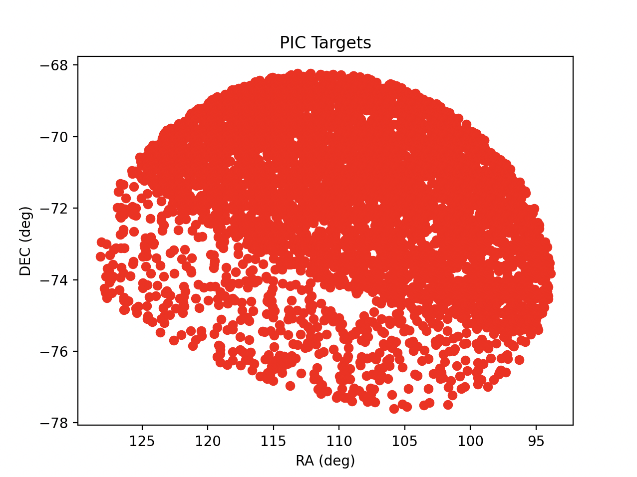
>>> results = plato.search_pic_target_go(target_name='Gaia DR3 5262913119040164480', radius=5)
Executed query:SELECT * FROM pic_go.pic_target_go WHERE 1=CONTAINS(POINT('ICRS', RAdeg, DEdeg),CIRCLE('ICRS', 111.43276923445, -73.19124693094, 5.0))
>>> plato.plot_plato_results(x=results['RAdeg'], y=results['DEdeg'], x_label='RA (deg)', y_label='DEC (deg)', plot_title='PIC Targets', color='red')
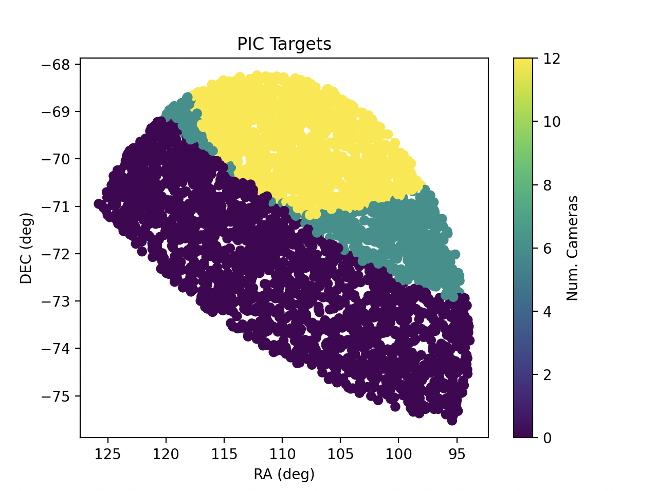
A third dimension can be drawn in the previous plot, assigning a value for the Z axis. This will generate the series with a colormap showing this third list of values. Please bear in mind that the colormap shall be available within Matplotlib collection.
>>> from astroquery.esa.plato import PlatoClass
>>> plato = PlatoClass()
>>> results = plato.search_pic_target_go(target_name='Gaia DR3 5262913119040164480', radius=5)
Executed query:SELECT * FROM pic_go.pic_target_go WHERE 1=CONTAINS(POINT('ICRS', RAdeg, DEdeg),CIRCLE('ICRS', 111.43276923445, -73.19124693094, 5.0))
>>> plato.plot_plato_results(x=results['RAdeg'], y=results['DEdeg'], z=results['BOLnCameraObsNCAM_T'], x_label='RA (deg)', y_label='DEC (deg)', z_label='Num. Cameras', plot_title='PIC Targets', color='viridis')
This method also allows to define x_error and y_error series, that will be added to the previous plot. As a result of
this method, the fig and ax objects from Matplotlib are returned, allowing the user to modify the plot in the desired way or
maybe update the current one, as they can be used as input parameters.
Reference/API#
astroquery.esa.plato Package#
European Space Astronomy Centre (ESAC) European Space Agency (ESA)
Classes#
|
This module connects with ESA Plato TAP |
|
Configuration parameters for |