ESA EUCLID Archive (astroquery.esa.euclid)#
The Euclid mission#
Euclid is a Medium class ESA mission to map the geometry of the dark Universe. The mission investigates the distance-redshift relationship and the evolution of cosmic structures. The space telescope is creating a detailed map of the large-scale structure of the Universe across space and time by observing billions of galaxies out to 10 billion light-years, across more than a third of the sky. It achieves this by measuring shapes and redshifts of galaxies and clusters of galaxies out to redshifts ~2, or equivalently to a look-back time of 10 billion years. It therefore explores how the Universe has expanded and how structure has formed over cosmic history, revealing more about the role of gravity and the nature of dark energy and dark matter.
Please take note of our guide on how to acknowledge and cite Euclid data if you use public Euclid data in your paper.
The PDR (Public Data Release) environment of the Euclid science archive holds the public data. Euclid Q1 data was publicly released on March 19, 2025. The main component of the Q1 data contains Level 2 data of a single visit (at the depth of the Euclid Wide Survey) over the Euclid Deep Fields (EDFs): 20 deg2 of the EDF North, 10 deg2 of EDF Fornax, and 23 deg2 of the EDF South. The deep fields will be visited multiple times during the mission.
By default, the object Euclid below makes use of the PDR environment:
>>> from astroquery.esa.euclid import Euclid
Astroquery.esa.euclid#
This Python module provides an Astroquery API to access to the metadata and datasets provided by the European Space Agency Euclid Archive using a TAP+ REST service. TAP+ is an extension of Table Access Protocol (TAP) specified by the International Virtual Observatory Alliance (IVOA) that incorporates dedicated user space capabilities (see Sect. 2 below). The TAP query language is Astronomical Data Query Language (ADQL). TAP provides two operation modes:
Synchronous: the server response is generated as soon as the request is received.
Asynchronous: the server starts a job that will execute the request. The first response to the request is a link with information about the job status.
On top of that, this package provides two access modes:
Public (default): The results generated by the anonymous ADQL queries are public, and deleted from the Archive 72 hours.
Authenticated: The ADQL queries and their outcomes remain in the user space until the user deletes them. In addition, authenticated users benefit from dedicated functionalities (see Sect 2 below).
There are limitations to the execution time and total output size that depend on the combination of operation and access modes - see the Gaia Archive FAQ: Why does my query time out after 90 minutes? Why is my query limited to 3 million rows? for details.
To reduce the verbosity (as well as complexity) of this document, the output of the code examples below has been trimmed and only the most relevant output lines are displayed. Whenever possible, the documentation points to the Astroquery.Gaia package that shares a similar architecture and methods with this module. For information about how to install the latest version of the Astroquery package, please visit the Astroquery page in PyPI.
Euclid data and data access#
Euclid Q1 contains different types of data, like catalogues (data tables), images, and (only the red part of the NISP) spectra. For details, please refer to the Data products in the science archive in the Euclid Archive Help , as well as the Q1 Data Product Definition Document (DPDD).
This Astroquery package is mostly geared to query and retrieve the data stored in the catalogues, but it also includes dedicated methods to retrieve the images and spectra (both stored as large FITS files). The latter are served via the DataLink IVOA protocol - see Sect. 3 below). It is also possible to directly access to these products (without having to retrieve them) using the “Euclid Q1” datalab that is publicly available in the ESA Datalabs e-science platform. Users aiming to analyse large Euclid datasets are encouraged to use this platform.
Table of contents:
Examples#
It is recommended checking the status of Euclid TAP before executing this module. To do this:
>>> from astroquery.esa.euclid import Euclid
>>> Euclid.get_status_messages()
1. Public access#
This is the access mode for non-registered (also known as “anonymous” in this document) users.
1.1. Metadata#
It is possible to access to the metadata (e.g., table names, sizes, descriptions, column names, etc.) of all the TAP tables stored in the Archive using the load_tables method. This feature allows to have a broad overview of the Archive content. To load only table names:
>>> tables = Euclid.load_tables(only_names=True, include_shared_tables=True)
INFO: Retrieving tables... [astroquery.utils.tap.core]
INFO: Parsing tables... [astroquery.utils.tap.core]
INFO: Done. [astroquery.utils.tap.core]
>>> print(f'* Found {len(tables)} tables')
* Found 98 tables
>>> print(*(table.name for table in tables), sep="\n")
catalogue.mer_catalogue
catalogue.mer_cutouts
catalogue.mer_morphology
catalogue.phz_classification
...
To load only one table and inspect its columns:
>>> raw_detector_table = Euclid.load_table('sedm.raw_detector')
>>> print(raw_detector_table)
TAP Table name: sedm.raw_detector
Description: None
Size (bytes): 0
Num. columns: 12
>>> print(*(column.name for column in raw_detector_table.columns), sep="\n")
crpix1
crpix2
crval1
...
1.2. Cone search#
The cone_search method allows to easily retrieve data around a projected circular region in a given sky location from a given catalogue. The example below shows how to launch a 0.5 degrees radius cone search around NGC 6505. By default, this method targets the “mer_catalogue” and its outcome is restricted to 50 rows.
>>> from astropy.coordinates import SkyCoord
>>> import astropy.units as u
>>> coord  = SkyCoord("17h51m07.4s +65d31m50.8s", frame='icrs')
>>> radius = u.Quantity(0.5, u.deg)
>>> job    = Euclid.cone_search(coordinate=coord, radius=radius, columns="*", async_job=True)
INFO: Query finished. [astroquery.utils.tap.core]
>>> cone_results    = job.get_results()
>>> print(f"Found {len(cone_results)} results")
Found 50 results
>>> print(cone_results)
basic_download_data_oid to_be_published ...          dist
                                        ...
----------------------- --------------- ... ----------------------
                    281               1 ... 0.00019856232836163457
                    281               1 ...   0.007812860952408775
                    281               1 ...   0.010825259849545266
                    281               1 ...   0.011471166543895434
...
To remove the row limitation one can set the Euclid.ROW_LIMIT to “-1”. The following example shows how to do this, as well as how to specify a target table. It also shows that the cone_search method accepts target names of coordinates, provided that the name is recognised by the Simbad, VizieR, or NED services.
>>> radius           = u.Quantity(0.2, u.deg)
>>> Euclid.ROW_LIMIT = -1
>>> job              = Euclid.cone_search(coordinate='NGC 6505', radius=radius, table_name="sedm.calibrated_frame", ra_column_name="ra", dec_column_name="dec", async_job=True, columns = ['ra', 'dec', 'datalabs_path', 'file_path', 'file_name', 'observation_id', 'instrument_name'])
INFO: Query finished. [astroquery.utils.tap.core]
>>> res              = job.get_results()
>>> print(f"* Found {len(res)} results")
* Found 14 results
>>> print(res)
     ra          dec     ... instrument_name         dist
    deg          deg     ...
------------ ----------- ... --------------- -------------------
267.99354663 65.60351547 ...            NISP 0.11414714851731637
267.99354663 65.60351547 ...             VIS 0.11414714851731637
267.99354663 65.60351547 ...            NISP 0.11414714851731637
267.99354663 65.60351547 ...             VIS 0.11414714851731637
...
Note
Once the table_name, and/or ra_column_name, and/or dec_column_name arguments are set, the default values are erased - this is a known issue.
Users are encouraged to use the cone_search instead of the query_object method. The latter makes use of the ADQL BOX function that is deprecated and can yield misleading results due to geometric projection effects.
1.3. Synchronous query#
This is the recommended access mode for queries that do not require excessive computation time and/or generate tables with less than 2,000 rows. The example below shows how to extract a subset of three sources with ellipticity larger than zero from the “mer_catalogue”:
>>> mer_cat_name = 'catalogue.mer_catalogue'
>>> query = f"SELECT TOP 3 object_id, right_ascension, declination, segmentation_area, ellipticity, kron_radius FROM {mer_cat_name} WHERE ellipticity > 0 ORDER BY object_id"
>>> job   = Euclid.launch_job(query)
>>> res   = job.get_results()
>>> print(res)
     object_id       right_ascension  ...     ellipticity        kron_radius
         NA                deg        ...          NA                pix
------------------- ----------------- ... ------------------- ------------------
-861556546086816217 86.15565466445506 ... 0.49623847007751465 31.741762161254883
-861553116086842109 86.15531167595952 ... 0.14531998336315155 19.158174514770508
-861547479086786330 86.15474795427782 ... 0.47604748606681824  46.28372573852539
The launch_job method returns a Job object. Its results can be extracted using the “get_results()” method, that generates an Astropy table object. The job status can be inspected by typing:
>>> print(job)
<Table length=3>
       name        dtype  unit                                                                          description
----------------- ------- ---- -------------------------------------------------------------------------------------------------------------------------------------------------------------
        object_id   int64   NA                                                                                                                               Euclid unique source identifier
  right_ascension float64  deg                                                                                      Source barycenter RA coordinate (SExtractor ALPHA_J2000) decimal degrees
      declination float64  deg                                                                                     Source barycenter DEC coordinate (SExtractor DELTA_J2000) decimal degrees
segmentation_area   int32  pix                                                                          Isophotal area of the source above the analysis threshold (SExtractor ISOAREA_IMAGE)
      ellipticity float64   NA A parametrization of how stretched an object is in the detection band, computed from the minor and major axes of the object itself (directly from SExtractor)
      kron_radius float64  pix                                       Major semi-axis (in pixels) of the elliptical aperture used for total (Kron) aperture photometry on the detection image
Jobid: None
Phase: COMPLETED
Owner: None
Output file: 43fa6c0a-2455-11f1-8a0e-e8ebd3edb7d7-TPDR-result.vot.gz
Results: None
Note that deleting the “TOP 3” string in the query above will return a table with 2,000 rows (sources).
1.4. Asynchronous query#
This is the recommended mode for queries that are expected to output more than 2,000 rows and that require substantial execution time (noting that all the queries time out after 7200 seconds). The query results are stored in the Archive (although for anonymous users the jobs are automatically deleted after 72 hours). The example below generates a cone search combined with a constraint applied to the ellipticity, and is similar to the first ADQL query example listed in the Euclid Archive (see its “Search/ADQL FORM” subtab). For more ADQL examples please have a look at the Gaia Archive Help content (in particular, the writing queries section).
>>> query = "SELECT right_ascension, declination, object_id, vis_det, det_quality_flag, flux_detection_total, flux_vis_sersic, segmentation_area, kron_radius, DISTANCE(267.78, 65.53, right_ascension, declination) AS dist FROM mer_catalogue WHERE DISTANCE(267.78, 65.53, right_ascension, declination) < 0.1 AND ellipticity > 0 order by right_ascension"
>>> job_async  = Euclid.launch_job_async(query, verbose=False)
INFO: Query finished. [astroquery.utils.tap.core]
>>> print(job_async)
<Table length=15129>
        name          dtype  unit                                                       description
-------------------- ------- ---- -----------------------------------------------------------------------------------------------------------------------
     right_ascension float64  deg                                                Source barycenter RA coordinate (SExtractor ALPHA_J2000) decimal degrees
         declination float64  deg                                               Source barycenter DEC coordinate (SExtractor DELTA_J2000) decimal degrees
           object_id   int64   NA                                                                                         Euclid unique source identifier
             vis_det   int16   NA              Flag to indicate if the source is detected in the VIS mosaic (1) or is only detected in the NIR mosaic (0)
    det_quality_flag   int16   NA                          Detection step flags that could indicate the possible corruption of the MAG_STARGAL_SEP values
flux_detection_total float64  uJy                                                           VIS or NIR stack band source total flux error (Kron aperture)
     flux_vis_sersic float64  uJy                                                                                VIS band source flux from the Sersic fit
   segmentation_area   int32  pix                                    Isophotal area of the source above the analysis threshold (SExtractor ISOAREA_IMAGE)
         kron_radius float64  pix Major semi-axis (in pixels) of the elliptical aperture used for total (Kron) aperture photometry on the detection image
                dist float64
Jobid: 97ab70be-2455-11f1-8a0e-e8ebd3edb7d7-TPDR
Phase: COMPLETED
Owner: None
Output file: async_20260320120906.vot
Results: None
>>> res  = job.get_results()
>>> print(res)
     object_id       right_ascension  ...     ellipticity        kron_radius
         NA                deg        ...          NA                pix
------------------- ----------------- ... ------------------- ------------------
-861556546086816217 86.15565466445506 ... 0.49623847007751465 31.741762161254883
-861553116086842109 86.15531167595952 ... 0.14531998336315155 19.158174514770508
-861547479086786330 86.15474795427782 ... 0.47604748606681824  46.28372573852539
1.5 Query on an ‘on-the-fly’ uploaded table#
This feature is present both in the synchronous and asynchronous queries. ‘On-the-fly’ queries allow the user to upload a table stored in VOTable format and perform a query on it in one single command. The uploaded tables are deleted after the query is complete. Alternatively, as a registered user it is possible to upload a table and store it in the user space (see Sect. 2 below). In the example below, the “my_table.xml” file is uploaded to the Archive via the “tap_upload” feature and then used to perform a combined (JOIN) operation with the mer_catalogue. Note the use of the “tap_upload” in the ADQL query.
>>> upload_resource = 'my_table.xml'
>>> query           = "SELECT mer.object_id, flux_vis_sersic, fwhm FROM tap_upload.table_test JOIN mer_catalogue AS mer USING (object_id)"
>>> job             = Euclid.launch_job(query, upload_resource=upload_resource, upload_table_name="table_test")
>>> res             = job.get_results()
>>> print(res)
    object_id        flux_vis_sersic          fwhm
------------------- ------------------- ------------------
2701338214642376775 0.12060821056365967 1.2710362672805786
2703077159642376093  0.8660399317741394 1.2481366395950317
2695939228642370900    6.01658296585083 1.2056430578231812
1.6. Getting products (FITS files)#
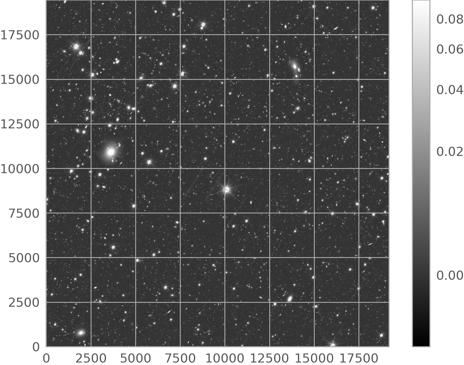
In addition to catalogues that can be queried via ADQL, the Euclid Archive also host the FITS files that contain the images and spectra generated by this mission. The example below shows how to download the Euclid (MER, background-subtracted) image of a given object proceeding in a two-step fashion.
Step 1: The “mosaic_product” TAP table that contains the names of the FITS files with the background-subtracted mosaic images (associated with the Euclid product: DpdMerBksMosaic) and their sky coverage (in its “fov” field) is queried using ADQL. Please note:
the “instrument_name” field that is used to select the “VIS” observations,
the variable “radius” that indicates the minimum distance between the target coordinates and the image edges, and
the combination of the INTERSECTS clause with the CIRCLE function. The target coordinates correspond to NGC 6505.
>>> radius   = 0.5/60.
>>> query    = f"""SELECT file_name, file_path, datalabs_path, instrument_name, filter_name, ra, dec, creation_date, product_type, patch_id_list, tile_index FROM q1.mosaic_product WHERE instrument_name='VIS' AND INTERSECTS(CIRCLE(267.7808, 65.5308, {radius}), fov)=1 ORDER BY file_name"""
>>> res      = Euclid.launch_job_async(query).get_results()
INFO: Query finished. [astroquery.utils.tap.core]
>>> print(res)
                                   file_name                                     ...
-------------------------------------------------------------------------------- ...
EUC_MER_BGSUB-MOSAIC-VIS_TILE102158889-F95D3B_20241025T024806.508980Z_00.00.fits ...
Step 2: The get_product method is used to download the fits file(s) listed in the “file_name” field included in the table returned in the previous step. The method returns the local path where the product(s) is saved.
Note
Given the size of the Euclid FITS images (~1.4 GB for the MER images and ~7 GB for calibrated VIS images) downloading individual files is time consuming (depending on the internet bandwith).
This step can be skipped if using ESA Datalabs (as direct access to the products is possible).
>>> file_name = res['file_name'][0]
>>> print("Downloading file:", file_name)
Downloading file: EUC_MER_BGSUB-MOSAIC-VIS_TILE102158889-F95D3B_20241025T024806.508980Z_00.00.fits
>>> file_name = res['file_name'][0]
>>> print("Downloading file:", file_name)
>>> path = Euclid.get_product(file_name=file_name, output_file=file_name)
Step 3: Open the FITS file and inspect its content.
>>> from astropy.io import fits
>>> import matplotlib.pyplot as plt
>>> from astropy.visualization import astropy_mpl_style, ImageNormalize, PercentileInterval, AsinhStretch,
>>> hdul = fits.open(path[0])
>>> image_data = hdul[0].data
>>>
>>> fig = plt.figure()
>>> plt.imshow(image_data, cmap='gray', origin='lower', norm=ImageNormalize(image_data, interval=PercentileInterval(99.1), stretch=AsinhStretch()))
>>> colorbar = plt.colorbar()
>>> hdul.close()
1.7. MER Cutouts#
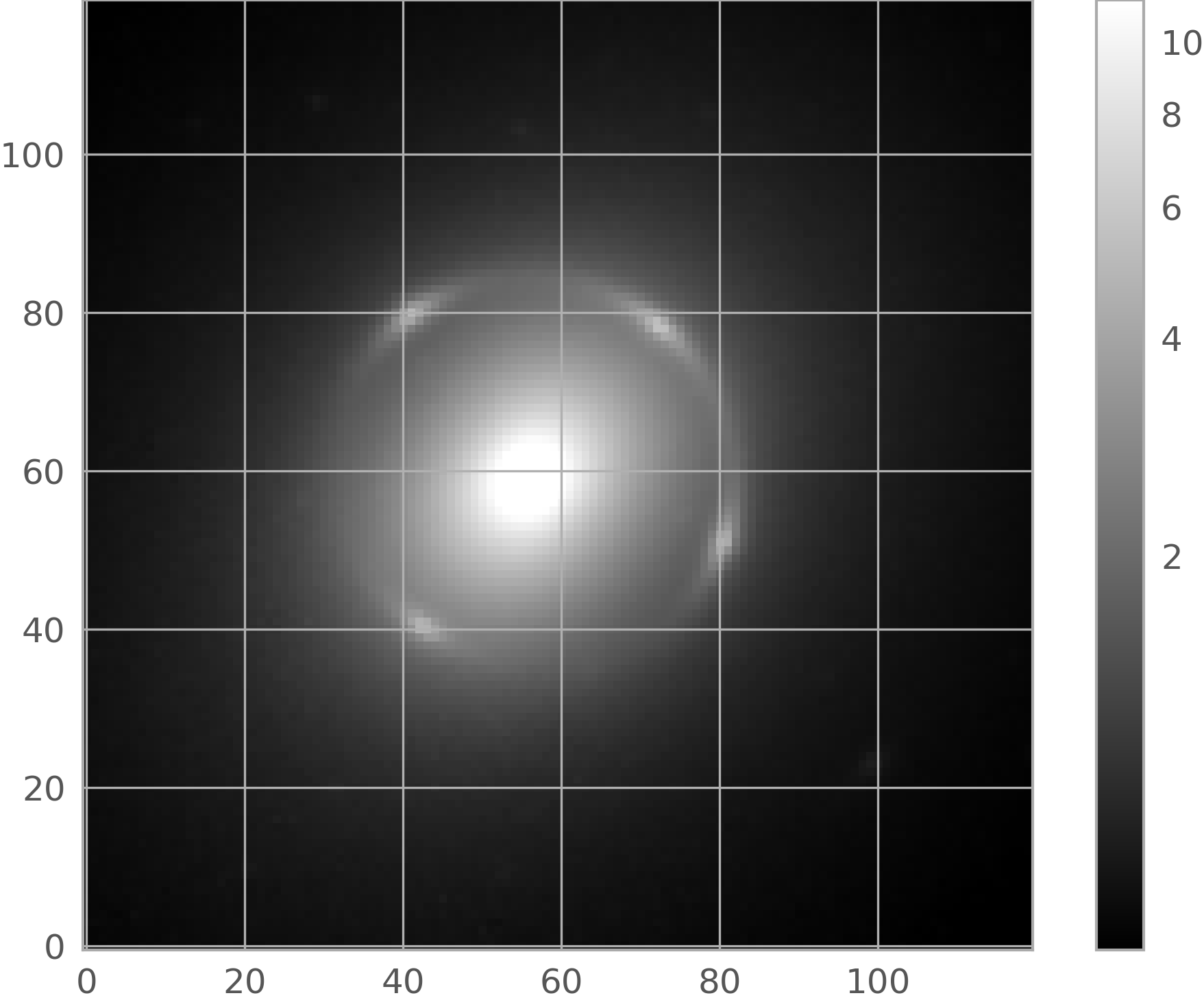
It is also possible to download just small portions of the MER (background subtracted) images. The get_cutout allows to download image cutouts and store them locally - for reference, downloading a 1’x1’cutout takes less than one second and the downloaded fits file weights ~5.5 MB. In the example below, the results of Step 1 are used to build the file_path of the MER background-subtracted mosaic, which is the only required product input for the get_cutout method. This method now only retrieves cutouts from MER mosaics.
Note
This method…
makes use of
astroquery.image_cutoutsto extract a cutout from a MER (background-subtracted) mosaic. It only supports MER mosaics. For more advanced use cases please see the Cutouts.ipynb notebook available in the Euclid Datalabs.accepts both Astropy SkyCoord coordinates and Simbad/VizieR/NED valid names (as string).
Download the cutout…
>>> file_path  = f"{res['file_path'][0]}/{res['file_name'][0]}"
>>> cutout_out = Euclid.get_cutout(file_path=file_path, coordinate='NGC 6505', radius= 0.1 * u.arcmin, output_file='ngc6505_cutout_mer.fits')
>>> cutout_out = cutout_out[0]
… and inspect its content:
>>> hdul       = fits.open(cutout_out)
>>> image_data = hdul[0].data
>>> fig = plt.figure()
>>> plt.imshow(image_data, cmap='gray', origin='lower', norm=ImageNormalize(image_data, interval=PercentileInterval(99.1), stretch=AsinhStretch()))
>>> colorbar = plt.colorbar()
>>> hdul.close()
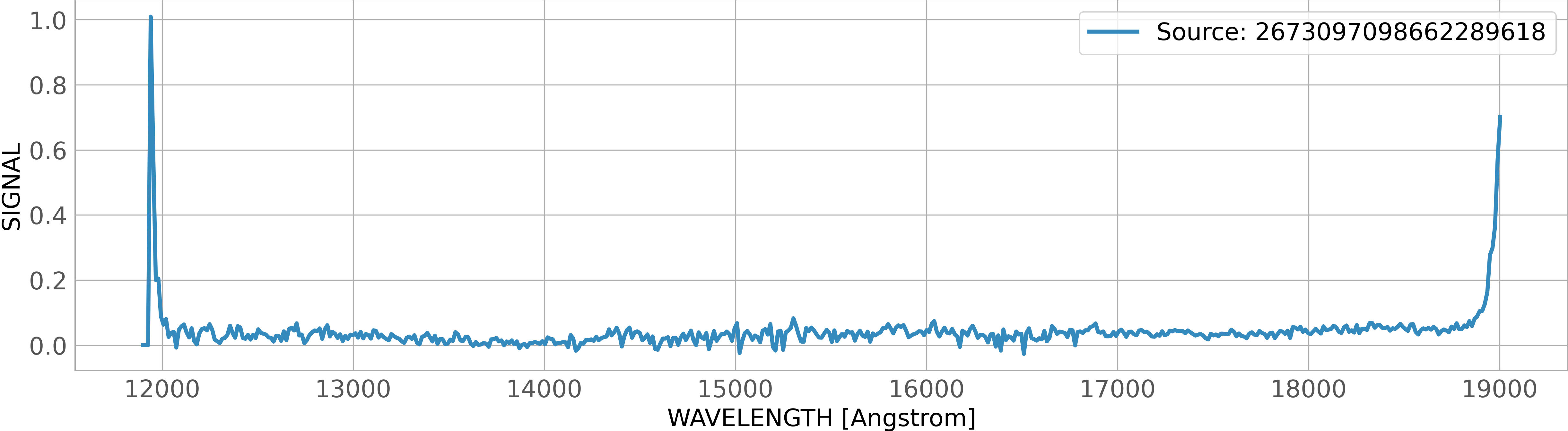
1.8 Spectra#
In the Archive the 1D Spectra data is served via the the Datalink (a data access protocol compliant with the IVOA architecture) service. Programmatically, this product is accessible via the get_spectrum method (see the Access to spectra section in the Archive help for more information about this product).
Note
As it happens when accessing to other Euclid products:
a two-step approach as detailed in Sect. 1.6 and 1.7 above is needed.
downloading of products is not needed when using ESA Datalabs.
Step 1: First, a list of sources that have associated spectra must be compiled. This information is available in the spectra_source table, that also includes the FITs file name and other metadata that is relevant if reading the spectra from Datalabs:
>>> query   = f"SELECT TOP 3 * FROM q1.spectra_source ORDER BY source_id"
>>> results = Euclid.launch_job_async(query).get_results()
INFO: Query finished. [astroquery.utils.tap.core]
>>> print(results)
combined_spectra_fk combined_spectra_product_fk ... to_be_published
------------------- --------------------------- ... ---------------
                306                       19410 ...               1
                306                       19410 ...               1
                306                       19410 ...               1
Alternatively, the get_datalinks method can be used to find out if a given source has associated spectra products, as well as to return its Datalabs-related metadata:
>>> result = Euclid.get_datalinks(ids=2707008224650763513, extra_options='METADATA')
>>> print(result)
           ID            linking_parameter ... hdu_index
                                           ...
------------------------ ----------------- ... ---------
sedm 2707008224650763513         SOURCE_ID ...      1602
sedm 2707008224650763513         SOURCE_ID ...      1602
Step 2: Retrieve the spectra associated to the list of sources compiled in the previous step using the get_spectrum method. The output is stored in a tabular fits file that can be open with the Astropy Table package as detailed below.
Download the spectra:
>>> inp_source = str(result['ID'][0]).replace('sedm ', '')  # Note: the input of get_spectrum must be a string.
>>> dl_out     = Euclid.get_spectrum(ids=inp_source, retrieval_type = "SPECTRA_RGS", verbose = True)
Spectra output file: /tmp/pytest-of-jfernandez/pytest-22/euclid_rst0/temp_20260320_145445/2707008224650763513.fits.zip
Retrieving data.
Data request: ID=sedm+2707008224650763513&SCHEMA=sedm&RETRIEVAL_TYPE=SPECTRA_RGS&USE_ZIP_ALWAYS=true&TAPCLIENT=ASTROQUERY
------>https
host = eas.esac.esa.int:443
context = /sas-dd/data
Content-type = application/x-www-form-urlencoded
200
Reading...
Done.
>>> print(f'Spectra downloaded and saved in: {dl_out}')
Spectra downloaded and saved in: ['/tmp/pytest-of-astroquery/pytest-23/euclid_rst0/temp_20260320_145608/SPECTRA_RGS-sedm 2707008224650763513.fits']
Read the spectra and convert it to Astropy table:
>>> from astropy.table import Table
>>> path_to_fits = dl_out[0]
>>> spec         = Table.read(dl_out[0], format = 'fits', unit_parse_strict='silent')
Plot it:
>>> fontsize = 18
>>> fig = plt.figure(figsize = [20,5])
>>> plt.plot(spec['WAVELENGTH'], spec['SIGNAL'], linewidth = 3, label = f"Source: {inp_source}")
>>> plt.xlabel(f"WAVELENGTH [{spec['WAVELENGTH'].unit}]", fontsize = fontsize)
>>> plt.ylabel('SIGNAL', fontsize = fontsize)
>>> plt.xticks(fontsize = fontsize)
>>> plt.yticks(fontsize = fontsize)
>>> plt.legend(fontsize = fontsize)
>>> plt.show()
2. Authenticated access#
Authenticated (registered) users have access to all the TAP+ capabilities (such as sharing tables, persistent jobs, and more). All the methods listed above are applicable to authenticated users, who also benefit from the the advantage of having the asynchronous jobs stored in the user area forever (until the user decides to remove them).
With Euclid DR1 the following features that are already available in the Astroquery.Gaia (see its “Section 2: Authenticated access”) package will also be available:
User space management: table upload and sharing capabilities.
Built-in cross-match functionality.
2.1. Login/Logout#
There are several ways to log in to the Euclid archive, as detailed below:
>>> from astroquery.esa.euclid import Euclid
>>> Euclid.login_gui()      # Login via graphic interface (pop-up window)
>>> Euclid.login()
>>> Euclid.login(user='<user_name>', password='<password>')
>>> Euclid.login(credentials_file='<path to credentials file>') # The file must contain just two rows: the username (first row) and the password.
>>> Euclid.logout()
2.2. Job deletion#
All the asynchronous jobs launched by registered users are stored in the user area, which can store up to 10 GB of jobs. Therefore, it is recommended to remove unnecessary jobs to avoid filling up the user quota. The example below shows how to delete all the jobs in the user area using the list_async_jobs and remove_jobs methods.
>>> Euclid.login()
>>> job_ids = [job.jobid for job in Euclid.list_async_jobs()]
>>> Euclid.remove_jobs(job_ids)
It is also possible to take advantage of the job metadata to delete all the jobs that were launched within a given time range as explained below.
First, use the load_async_job method to download the metadata of the async jobs stored in the user space:
>>> job_obj  = [Euclid.load_async_job(jobid=jobid) for jobid in job_ids]
>>> job_ids  = [job.jobid        for job in job_obj]
>>> dates    = [job.creationTime for job in job_obj]
Second, create a dataframe that contains the jobid and date information:
>>> df              = pd.DataFrame.from_dict({'job_id':job_ids, 'fulldate':dates})
>>> df['date_time'] = pd.to_datetime(df['fulldate'])
>>> df['date']      = df['date_time'].dt.date
>>> df['hour_UTC']  = df['date_time'].dt.hour
Finally, extract the job id’s included in a given time range (in the example below, all the jobs stored since 2024-10-01 at 7 hours UTC) and delete them:
>>> subset          = df[(df['date'] == datetime.date(2024,10,1)) & (df['hour_UTC'].isin([7]))]
>>> jobs_to_delete  = subset['job_id'].to_list()
>>> Euclid.remove_jobs(jobs_to_delete)
Appendix#
The following table summarises the available values of the parameters of the method get_scientific_product_list.
category |
group |
product_type |
description |
|---|---|---|---|
‘Internal Data Products’ |
‘SEL Wide Main’ |
‘DpdLE3IDSELIDCatalog’ |
|
‘Internal Data Products’ |
‘SEL Wide’ |
‘DpdLE3IDSELIDSubsampledCatalog’ |
|
‘Internal Data Products’ |
‘VMSP Group’ |
‘DpdLE3IDVMSPConfiguration’ |
VMSP Configuration |
‘Internal Data Products’ |
‘VMSP Group’ |
‘DpdLE3IDVMSPDetectionModel’ |
VMSP ID Detection Model |
‘Internal Data Products’ |
‘VMSP Group’ |
‘DpdLE3IDVMSPDistModel’ |
VMSP Distribution Model |
‘Internal Data Products’ |
‘VMSP Group’ |
‘DpdLE3IDVMSPRandomCatalog’ |
Random Catalog Product |
‘Internal Data Products’ |
‘SEL Config/Stats’ |
‘DpdLE3IDSELIDStatistics’ |
SEL-ID Purity and completeness statistics |
‘Internal Data Products’ |
‘SEL Config/Stats’ |
‘DpdLE3IDSELConfigurationSet’ |
SEL Configuration |
‘Internal Data Products’ |
‘External Data Products’ |
‘LE3-ED configuration catalog’ |
LE3-ED configuration catalog |
‘Internal Data Products’ |
‘External Data Products’ |
‘LE3-ED match catalog’ |
‘DpdLE3edMatchedCatalog’ |
‘Weak Lensing Products’ |
‘2PCF’ |
‘DpdTwoPCFWLCOSEBIFilter’ |
This product contains COSEBI filters |
‘Weak Lensing Products’ |
‘2PCF’ |
‘DpdTwoPCFWLParamsCOSEBIShearShear2D’ |
This product contains parameters to compute the |
‘Weak Lensing Products’ |
‘2PCF’ |
‘DpdTwoPCFWLParamsClPosPos2D’ |
This product contains parameters to compute the tomographic |
‘Weak Lensing Products’ |
‘2PCF’ |
‘DpdTwoPCFWLParamsPEBPosShear2D’ |
This product contains parameters to compute the |
‘Weak Lensing Products’ |
‘2PCF’ |
‘DpdTwoPCFWLParamsPEBShearShear2D’ |
This product contains parameters to compute the |
‘Weak Lensing Products’ |
‘2PCF’ |
‘DpdTwoPCFWLParamsPosPos2D’ |
Input parameters to compute tomographic angular 2PCF. |
‘Weak Lensing Products’ |
‘2PCF’ |
‘DpdTwoPCFWLParamsPosShear2D’ |
Input parameters to compute the tomographic galaxy-galaxy lensing 2PCF. |
‘Weak Lensing Products’ |
‘2PCF’ |
‘DpdTwoPCFWLParamsShearShear2D’ |
Input parameters to compute tomographic cosmic shear 2PCF. |
‘Weak Lensing Products’ |
‘2PCF’ |
‘DpdTwoPCFWLCOSEBIShearShear2D’ |
Tomographic cosmic shear COSEBI modes. |
‘Weak Lensing Products’ |
‘2PCF’ |
‘DpdTwoPCFWLClPosPos2D’ |
This product contains the tomographic angular power spectra |
‘Weak Lensing Products’ |
‘2PCF’ |
‘DpdTwoPCFWLPEBPosShear2D’ |
Tomographic galaxy-galaxy lensing E/B power spectra |
‘Weak Lensing Products’ |
‘2PCF’ |
‘DpdTwoPCFWLPEBShearShear2D’ |
Tomographic cosmic shear E/B power spectra. |
‘Weak Lensing Products’ |
‘2PCF’ |
‘DpdTwoPCFWLPosPos2D’ |
Tomographic angular 2PCF. |
‘Weak Lensing Products’ |
‘2PCF’ |
‘DpdTwoPCFWLPosShear2D’ |
Tomographic galaxy galaxy lensing 2PCF. |
‘Weak Lensing Products’ |
‘2PCF’ |
‘DpdTwoPCFWLShearShear2D’ |
Tomographic cosmic shear 2PCF. |
‘Weak Lensing Products’ |
‘2PCF’ |
‘DpdCovarTwoPCFWLParams’ |
This product contains resampling parameters to compute the covariance matrices. |
‘Weak Lensing Products’ |
‘2PCF’ |
‘DpdCovarTwoPCFWLClPosPos2D’ |
Covariance of Tomographic Angular Power Spectra |
‘Weak Lensing Products’ |
‘2PCF’ |
‘DpdCovarTwoPCFWLCOSEBIShearShear2D’ |
Covariance of Tomographic Cosmic Shear COSEBI |
‘Weak Lensing Products’ |
‘2PCF’ |
‘DpdCovarTwoPCFWLPEBPosShear2D’ |
Cov. of Tomo. Galaxy-Galaxy Lensing EB Power Spectra |
‘Weak Lensing Products’ |
‘2PCF’ |
‘DpdCovarTwoPCFWLPEBShearShear2D’ |
Covariance of Tomographic Cosmic Shear EB Power Spectra |
‘Weak Lensing Products’ |
‘2PCF’ |
‘DpdCovarTwoPCFWLPosPos2D’ |
Covariance of Tomographic Angular Correlation |
‘Weak Lensing Products’ |
‘2PCF’ |
‘DpdCovarTwoPCFWLPosShear2D’ |
Cov. of Tomographic Galaxy-Galaxy Lensing Correlation |
‘Weak Lensing Products’ |
‘2PCF’ |
‘DpdCovarTwoPCFWLShearShear2D’ |
Covariance of Tomographic Cosmic Shear Correlation |
‘Weak Lensing Products’ |
‘2PCF’ |
‘DpdCovarTwoPCFWLResampleCOSEBIShearShear2D’ |
This product contains a list of resampled tomographic cosmic shear COSEBI modes. |
‘Weak Lensing Products’ |
‘2PCF’ |
‘DpdCovarTwoPCFWLResampleClPosPos2D’ |
This product contains a list of resampled tomographic angular power spectrum. |
‘Weak Lensing Products’ |
‘2PCF’ |
‘DpdCovarTwoPCFWLResamplePEBPosShear2D’ |
This product contains a list of resampled tomographic galaxy-galaxy lensing E/B power spectra. |
‘Weak Lensing Products’ |
‘2PCF’ |
‘DpdCovarTwoPCFWLResamplePEBShearShear2D’ |
This product contains a list of resampled tomographic cosmic shear E/B power spectra. |
‘Weak Lensing Products’ |
‘2PCF’ |
‘DpdCovarTwoPCFWLResamplePosPos2D’ |
This product contains a list of resampled tomographic galaxy-galaxy lensing correlation function. |
‘Weak Lensing Products’ |
‘2PCF’ |
‘DpdCovarTwoPCFWLResamplePosShear2D’ |
This product contains a list of resampled tomographic galaxy-galaxy lensing correlation function. |
‘Weak Lensing Products’ |
‘2PCF’ |
‘DpdCovarTwoPCFWLResampleShearShear2D’ |
This product contains a list of resampled tomographic cosmic shear 2PCF. |
‘Weak Lensing Products’ |
‘PK’ |
‘DpdPKWLAlms’ |
Data product that contains the alms generated by PK-WL. |
‘Weak Lensing Products’ |
‘PK’ |
‘DpdPKWLCovMatrix2D’ |
This product contains the covariance matrix of angular power spectra. |
‘Weak Lensing Products’ |
‘PK’ |
‘DpdPKWLEstimate2D’ |
This product contains the tomographic angular clustering power spectra. |
‘Weak Lensing Products’ |
‘PK’ |
‘DpdPKWLMaps’ |
Data product that contains the FITS file with maps generated by PK-WL. |
‘Weak Lensing Products’ |
‘PK’ |
‘DpdPKWLMixingMatrix2D’ |
This product contains the mixing matrix components. |
‘Weak Lensing Products’ |
‘2D-MASS’ |
‘DpdTwoDMassParamsConvergenceClusters’ |
This product contains input parameters to compute the 2D convergence maps for clusters studies. |
‘Weak Lensing Products’ |
‘2D-MASS’ |
‘DpdTwoDMassParamsConvergencePatch’ |
This product contains inputs to compute the 2D convergence maps for one or several patches. |
‘Weak Lensing Products’ |
‘2D-MASS’ |
‘DpdTwoDMassParamsConvergencePatchesToSphere’ |
This product contains inputs to compute the 2D convergence maps on the sphere. |
‘Weak Lensing Products’ |
‘2D-MASS’ |
‘DpdTwoDMassParamsConvergenceSphere’ |
This product contains inputs to compute the 2D convergence maps on the sphere. |
‘Weak Lensing Products’ |
‘2D-MASS’ |
‘DpdTwoDMassParamsPeakCatalogConvergence’ |
This product contains inputs to perform peak counting on a convergence map. |
‘Weak Lensing Products’ |
‘2D-MASS’ |
‘DpdTwoDMassParamsPeakCatalogMassAperture’ |
This product contains inputs to perform peak counting on shear catalog for one or several patches |
‘Weak Lensing Products’ |
‘2D-MASS’ |
‘DpdTwoDMassConvergenceClusters’ |
E/B Convergence Maps for Clusters |
‘Weak Lensing Products’ |
‘2D-MASS’ |
‘DpdTwoDMassConvergencePatchesToSphere’ |
MultiPatch-Based E/B Convergence Maps for Large field |
‘Weak Lensing Products’ |
‘2D-MASS’ |
‘DpdTwoDMassConvergencePatch’ |
E/B Convergence Maps for Small Field |
‘Weak Lensing Products’ |
‘2D-MASS’ |
‘DpdTwoDMassConvergenceSphere’ |
Spherical E/B Convergence Maps |
‘Weak Lensing Products’ |
‘2D-MASS’ |
‘DpdTwoDMassPeakCatalog’ |
Peak Catalog |
‘Galaxy Clustering Products’ |
‘2PCF_PK’ |
‘DpdLE3gcPkCross’ |
Cross [Power Spectrum Multipoles and Window Product] |
‘Galaxy Clustering Products’ |
‘2PCF_PK’ |
‘DpdLE3gcPkDOA’ |
DOA [Power Spectrum Multipoles, 2Dpolar, 2Dcart and Window Product] |
‘Galaxy Clustering Products’ |
‘2PCF_PK’ |
‘DpdLE3gcPkYam’ |
Yamamoto [Power Spectrum Multipoles and Window Product] |
‘Galaxy Clustering Products’ |
‘2PCF_PK’ |
‘DpdLE3gcTwoPointAutoCorr’ |
1D [Angle-averaged Auto-correlation Product] |
‘Galaxy Clustering Products’ |
‘2PCF_PK’ |
‘DpdLE3gcTwoPointAutoCorrCart’ |
2D Cartesian [2D Cartesian and Projected Auto-corr. Product] |
‘Galaxy Clustering Products’ |
‘2PCF_PK’ |
‘DpdLE3gcTwoPointAutoCorrPol’ |
2D Polar [2D Polar and Multipole Auto-correlation Product] |
‘Galaxy Clustering Products’ |
‘2PCF_PK’ |
‘DpdLE3gcTwoPointCrossCorr’ |
1D [Angle-averaged Cross-correlation Product] |
‘Galaxy Clustering Products’ |
‘2PCF_PK’ |
‘DpdLE3gcTwoPointCrossCorrCart’ |
2D Cartesian [2D Cartesian and Projected Cross-corr. Product] |
‘Galaxy Clustering Products’ |
‘2PCF_PK’ |
‘DpdLE3gcTwoPointCrossCorrPol’ |
2D Polar [2D Polar and Multipole Cross-correlation Product] |
‘Galaxy Clustering Products’ |
‘2PCF_PK’ |
‘DpdLE3gcTwoPointRecAutoCorr’ |
1D [Post-reconstruction Angle-averaged Auto-correlation Product] |
‘Galaxy Clustering Products’ |
‘2PCF_PK’ |
‘DpdLE3gcTwoPointRecAutoCorrCart’ |
2D Cartesian [Post-reconstruction 2D Cartesian and Projected Auto-correlation Product] |
‘Galaxy Clustering Products’ |
‘2PCF_PK’ |
‘DpdLE3gcTwoPointRecAutoCorrPol’ |
2D Polar [Post-reconstruction 2D Polar and Multipole Auto-correlation Product] |
‘Galaxy Clustering Products’ |
‘2PCF_PK’ |
‘DpdLE3gcTwoPointRecCrossCorr’ |
1D [Post-reconstruction Angle-averaged Cross-corr. Product] |
‘Galaxy Clustering Products’ |
‘2PCF_PK’ |
‘DpdLE3gcTwoPointRecCrossCorrCart’ |
2D Cartesian [Post-reconstruction 2D Cartesian and Projected Cross-correlation Product] |
‘Galaxy Clustering Products’ |
‘2PCF_PK’ |
‘DpdLE3gcTwoPointRecCrossCorrPol’ |
2D Polar [Post-reconstruction 2D Polar and Multipole Cross-correlation Product] |
‘Galaxy Clustering Products’ |
‘3PCF_BK’ |
‘DpdLE3gcThreePointAll’ |
3PCF Triplets “ALL” Product |
‘Galaxy Clustering Products’ |
‘3PCF_BK’ |
‘DpdLE3gcThreePointSin’ |
3PCF Correlation “SINGLE” Product |
‘Galaxy Clustering Products’ |
‘3PCF_BK’ |
‘DpdLE3gcBkMonopole’ |
Bispectrum Product Monopole |
‘Galaxy Clustering Products’ |
‘3PCF_BK’ |
‘DpdLE3gcBkMultipole’ |
Bispectrum Product Multipoles |
‘Galaxy Clustering Products’ |
‘CM-2PCF’ |
‘DpdLE3gcCovmatTwoPointCov1D’ |
Output, 1D [Covariance Matrix of the Angle-averaged Auto-correlation Product] |
‘Galaxy Clustering Products’ |
‘CM-2PCF’ |
‘DpdLE3gcCovmatTwoPointCov2Dcart’ |
Output, 2D cartesian [Covariance Matrix of the 2D Cartesian 2PCF Product] |
‘Galaxy Clustering Products’ |
‘CM-2PCF’ |
‘DpdLE3gcCovmatTwoPointCov2Dpol’ |
Output, 2D Polar [Covariance Matrix of the 2D Polar 2PCF Product] |
‘Galaxy Clustering Products’ |
‘CM-2PCF’ |
‘DpdLE3gcCovmatTwoPointCovMu’ |
Output, Covariance Matrix of the Multipoles 0, 1, 2, 3, 4 2PCF Product |
‘Galaxy Clustering Products’ |
‘CM-2PCF’ |
‘DpdLE3gcCovmatTwoPointCovPro’ |
Output, Projected [Covariance Matrix of the Projected 2PCF Product] |
‘Galaxy Clustering Products’ |
‘CM-PK’ |
‘DpdLE3gcCovmatPKCov1D’ |
Output, Covariance Matrix of the Power Spectrum 0, 1, 2, 3, 4 multipoles Product |
‘Galaxy Clustering Products’ |
‘CM-PK’ |
‘DpdLE3gcCovmatPKCov2Dcart’ |
Output, Covariance Matrix of the Power Spectrum 2D Cartesian Product |
‘Galaxy Clustering Products’ |
‘CM-PK’ |
‘DpdLE3gcCovmatPKCov2Dpol’ |
Output, Covariance Matrix of the Power Spectrum 2D Polar Product |
‘Clusters of Galaxies’ |
‘GrpCatalog |
‘DpdLE3clAMICOModel’ |
This product contains the Model for AMICO |
‘Clusters of Galaxies’ |
‘GrpCatalog |
‘DpdLE3clDetMergeParams’ |
This product contains the input parameters for DET |
‘Clusters of Galaxies’ |
‘GrpCatalog |
‘DpdLE3clDetOnMockParams’ |
This product contains the input parameters for DET_ON_MOCK pipeline |
‘Clusters of Galaxies’ |
‘GrpCatalog |
‘DpdLE3clDetInputParams’ |
This product contains the input parameters for DEt |
‘Clusters of Galaxies’ |
‘GrpCatalog |
‘DpdLE3clAmicoAux’ |
DET-CL AMICO auxiliary Data Product |
‘Clusters of Galaxies’ |
‘GrpCatalog |
‘DpdLE3clAssociations’ |
This output product contains the catalog of associations galaxy to clusters |
‘Clusters of Galaxies’ |
‘GrpCatalog |
‘DpdLE3clPzwavAux’ |
DET-CL PZWAV auxiliary Data Product |
‘Clusters of Galaxies’ |
‘GrpCatalog |
‘DpdLE3clPZWAVDensity’ |
This output product contains the intermediate Product “Density Map” from DET-CL/PZWAV |
‘Clusters of Galaxies’ |
‘GrpCatalog |
‘DpdLE3clDetClusters’ |
This output product contains the catalog of candidate clusters from DET-CL |
‘Clusters of Galaxies’ |
‘GrpCatalog |
‘DpdLE3FullDet’ |
This output product contains the merged catalog of candidate clusters |
‘Clusters of Galaxies’ |
‘GrpCatalog |
‘DpdLE3clCatMergeParams’ |
This product contains the input parameters for the merging in CAT-CL |
‘Clusters of Galaxies’ |
‘GrpCatalog |
‘DpdLE3clCATParams’ |
This product contains the configuration parameters for LE3 CAT-CL |
‘Clusters of Galaxies’ |
‘GrpCatalog |
‘DpdLE3clCcpInputParams’ |
This product contains the input parameters for Cluster Characterization Pipeline |
‘Clusters of Galaxies’ |
‘GrpCatalog |
‘DpdLE3clRichMembers’ |
Galaxy Membership Output Product |
‘Clusters of Galaxies’ |
GrpCatalog |
‘DpdLE3clZClParams’ |
This product contains the configuration parameters for LE3 Z-CL |
‘Clusters of Galaxies’ |
‘GrpCatalog |
‘DpdLE3clGlueMatchParams’ |
This product contains the input parameters for the glue-match pipeline |
‘Clusters of Galaxies’ |
‘GrpCatalog |
‘DpdLE3clMockGlueMatchParams’ |
This product contains the input parameters for the mock glue-match pipeline |
‘Clusters of Galaxies’ |
‘GrpCatalog’ |
‘DpdLE3clGlueMatchParams’ |
This product contains the input parameters for the glue-match pipeline. |
‘Clusters of Galaxies’ |
‘GrpCOMB’ |
‘DpdLE3clCombConfigurationSet’ |
Configuration information for COMB-CL pipelines |
‘Clusters of Galaxies’ |
‘GrpCOMB’ |
‘DpdLE3clCombRedSheProf’ |
Output Reduced shear profiles |
‘Clusters of Galaxies’ |
‘GrpCOMB’ |
‘DpdLE3clCombUCovRedSheProf’ |
Output Uncertainty Covariance matrix of the reduced |
‘Clusters of Galaxies’ |
‘GrpCOMB’ |
‘DpdLE3clCombWLME’ |
Output Weak lensing mass estimates |
‘Clusters of Galaxies’ |
‘GrpCOMB’ |
‘DpdLE3clCombCovMatDeltaSigmaCosmoDep’ |
This output product contains the stacking |
‘Clusters of Galaxies’ |
‘GrpCOMB’ |
‘DpdLE3clCombCovMatReducedShearCosmoDep’ |
This output product contains the stacking covariance matrix of the reduced shear derived with a cosmology dependent binning. |
‘Clusters of Galaxies’ |
‘GrpCOMB’ |
‘DpdLE3clCombCovMatReducedShearCosmoIndep’ |
This output product contains the stacking covariance matrix of the reduced shear derived with a cosmology independent binning. |
‘Clusters of Galaxies’ |
‘GrpCOMB’ |
‘DpdLE3clCombStackingCosmoDep’ |
This output product contains the stacking cosmology dependent binning. |
‘Clusters of Galaxies’ |
‘GrpCOMB’ |
‘DpdLE3clCombStackingCosmoInd’ |
This output product contains the stacking cosmology independent binning. |
‘Clusters of Galaxies’ |
‘GrpSEL’ |
‘DpdLE3clSelRandomParams’ |
This output product contains the configuration parameters for SEL-CL to create the random catalogue |
‘Clusters of Galaxies’ |
‘GrpSEL’ |
‘DpdLE3clSelSelFuncInputParams’ |
This product contains the input parameters for SEL SelFunc |
‘Clusters of Galaxies’ |
‘GrpSEL’ |
‘DpdLE3clSelSinfoniaIniClMockInputParams’ |
This product contains the input parameters for SEL Sinfonia Cluster Mock pipeline |
‘Clusters of Galaxies’ |
‘GrpSEL’ |
‘DpdLE3clSelSinfoniaMockInputParams’ |
This product contains the input parameters for SEL Sinfonia Mock pipeline |
‘Clusters of Galaxies’ |
‘GrpSEL’ |
‘DpdLE3clSelSelFunc’ |
This output product contains the selection function of the galaxy cluster detections |
‘Clusters of Galaxies’ |
‘GrpSEL’ |
‘DpdLE3clSinfoniaEllipticity’ |
This output product contains the file for the ellipticity |
‘Clusters of Galaxies’ |
‘GrpSEL’ |
‘DpdLE3clSelSubSample’ |
Clusters Subsample Output Product |
‘Clusters of Galaxies’ |
‘GrpSEL’ |
‘DpdLE3clRedshiftDistrib’ |
Redshift distribution of detections |
‘Clusters of Galaxies’ |
‘GrpSEL’ |
‘DpdLE3clSelRandom’: |
Random for the CL clustering codes |
‘Clusters of Galaxies’ |
‘GrpSEL’ |
‘DpdLE3clMatchForSelParams’ |
This product contains the input parameters for the match-for-sel pipeline |
‘Clusters of Galaxies’ |
‘GrpSEL’ |
‘DpdLE3clMockClusters’ |
This output product contains the catalog of mock clusters |
‘Clusters of Galaxies’ |
‘GrpClustering’ |
‘DpdLE3clTwoPointAutoCorrPol’ |
Cluster Clustering Two Point Correlation 2D polar data product |
‘Clusters of Galaxies’ |
‘GrpClustering’ |
‘DpdLE3clCovmatTwoPointCov2’ |
Cluster Clustering Covariance Matrix 2PCF 2D polar data product |
‘Clusters of Galaxies’ |
‘GrpClustering’ |
‘DpolDpdLE3clCovmatPKCov1’ |
|
‘Clusters of Galaxies’ |
‘GrpClustering’ |
‘DDpdLE3clPkDOA’ |
|
‘Clusters of Galaxies’ |
‘GrpClustering’ |
‘DpdLE3clPkYam’ |
Cluster Clustering Power Spectrum Yamamoto data product |
‘Clusters of Galaxies’ |
‘GrpLMF’ |
‘DpdLE3clLMFParams’ |
This product contains the configuration parameters for LE3 LMF-CL |
‘Clusters of Galaxies’ |
‘GrpLMF’ |
‘DpdLE3clLMFOutput’ |
This product contains the output for LE3_CL LMF PF |
‘Clusters of Galaxies’ |
‘GrpTiling’ |
‘DpdLE3clCLTile’ |
This product contains the information describing a CL tile |
‘Clusters of Galaxies’ |
‘GrpTiling’ |
‘DpdLE3clCommon’ |
Common data product for CL |
‘Clusters of Galaxies’ |
‘GrpTiling’ |
‘DpdLE3clConfigurationSet’ |
Generic configuration information for CL PFs |
‘PHZ’ |
‘PHZ’ |
‘DpdBinMeanRedshift’ |
|
‘PHZ’ |
‘PHZ’ |
‘DpdReferenceSample’ |
|
‘PHZ’ |
‘PHZ’ |
‘DpdTomographicBins’ |
Reference/API#
astroquery.esa.euclid Package#
European Space Astronomy Centre (ESAC) European Space Agency (ESA)
Classes#
|
Constructor for EuclidClass. |
|
Configuration parameters for |